EXPOSURE VARIABILITY

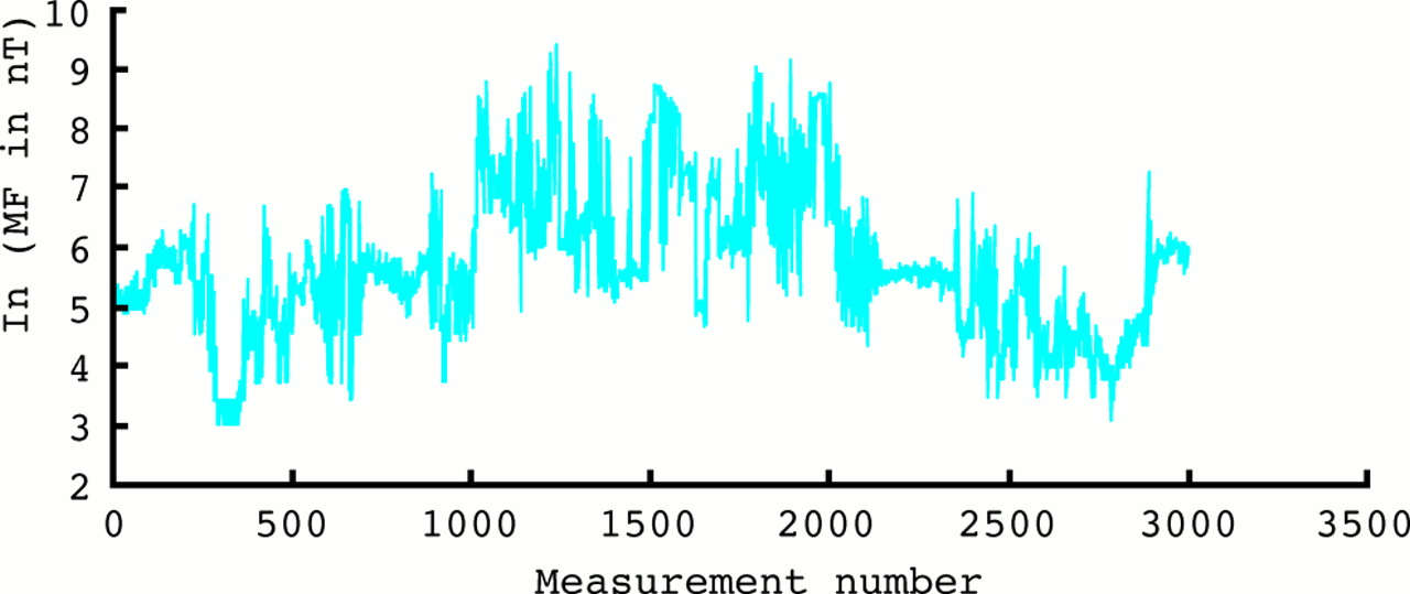
Measurements of workplace exposures are crucial not only for evaluations of potential health risks, but also for their subsequent reduction through efficient control measures. When designing measurement strategies the generally large sources of exposure variability should be appreciated in order to design efficient and effective protocols. Exposure concentrations are known to be extremely variable, especially within a day over short averaging times (fig 2). On the other hand, long term decreasing trends in exposure concentrations at an average rate of 6% per annum have recently been described for workplace exposures in western industrialised countries.³ Therefore, variability in yearly average concentrations will be much smaller than variability in eight hour shift long measurements that have been estimated to vary between 3–4000 fold.⁴ For 10 second point estimated levels of magnetic field exposure for workers in the utility industry it was estimated that they on average varied an additional 50 fold.⁵ (fig 2).

The extent to which exposures vary depends on many factors.⁴ Some of these are concerned with the agent itself, but the majority are linked to work content, tasks performed, production, and environment characteristics. In general, analytical and sampling errors play a minor role in overall exposure variability.

Recently, a database with repeated shift long inhalation exposure measurements from a variety of workplaces and industries was constructed and analysed. For a group of workers (defined by job title and location) it was estimated that personal mean inhalation exposures fall on average within a fivefold range. In a temporal sense, daily exposures were estimated to fall on average within a 15-fold range.⁴ Even more recently, a similar database was built for dermal exposure and again there was evidence of a larger temporal component than personal component.⁶ Spatial variability (differences in exposure between body locations) was estimated to be even more prominent.

Breakdowns of variance components by industry, production, and environmental factors revealed important differences that should be taken into account when designing measurement strategies (box 4). For example, for outdoor exposures temporal effects tended to outweigh completely minor differences between workers in the same group. For crews of paving workers with distinct jobs this was recently corroborated. Their exposure to bitumen fume appeared to be uniform despite differences in jobs performed. Temporal variability of their exposure was up to a 30-fold range.⁷

STANDARD MEASUREMENT STRATEGIES FOR COMPLIANCE WITH EIGHT HOUR TIME WEIGHTED AVERAGE LIMIT VALUES

Traditionally worst case sampling strategies were thought to be very efficient, because they focused measurements upon situations where they were most needed. This approach of sampling the “maximum risk employee” has been widely propagated from the 1970s onwards, primarily as a result of the appearance of the National Institute of Occupational Safety and Health (NIOSH) occupational exposure sampling strategy manual.⁸ Similar considerations also form the basis of the European Norm 689 Guidance for the assessment of exposure to chemical agents for comparison with limit values.⁹ However, because of the restrictions typical of these measurement strategies, they produce incomplete and upwardly biased pictures of exposure concentrations. In addition, these measurement strategies assume implicitly that workers sharing the same environment and tasks are similarly exposed and therefore experience the same risks. Given modern understanding of exposure variability this constitutes a far too rosy and simplistic picture.

EFFICIENT MEASUREMENT STRATEGY FOR HAZARD CONTROL

Recently, a new measurement strategy for evaluation of long term average concentrations has been developed that incorporates the notion that workers are not necessarily similarly exposed even though they may work in the same environment and basically perform similar tasks.^10,11 George et al described a striking example of this phenomenon in a car manufacturing plant, where workers were exposed to isopropyl alcohol while wiping an automobile in a heavily ventilated downdraft booth (90 nominal air changes per hour).¹² Even under these well controlled circumstances there appeared to be an almost fourfold difference in long term average exposure between two workers because of differences in body length, resulting in different distances to the exposure source and consequently different mean exposure concentrations.

In the newly developed measurement strategy, sampling is performed on randomly chosen workers from an a priori identified group of workers (observational group) on repeated days.^10,11 A schematic overview of this measurement protocol is presented in fig 3. After this initial sampling effort the protocol fits a random effects analysis of variance (ANOVA) model to the logged exposure data, and the goodness-of-fit of this model is checked by a graphical procedure. If the fit is acceptable for a given observational group the group is regarded as monomorphic and subsequently tested for overexposure. If the group cannot be considered to be monomorphic an alternative grouping should be attempted. For a monomorphic group the estimated statistical parameters are used to assess whether the probability is acceptably small that a randomly selected worker would be overexposed (that is, a randomly selected worker's mean exposure is above an occupational exposure limit). For groups of workers whose exposure were found to be unacceptable, re-sampling is suggested in some cases to increase the power of the test for declaring existing exposures acceptable. If re-sampling and consequent re-testing do not result in an acceptable situation the protocol tests the uniformity of the exposure (that is, whether workers have essentially the same mean exposure) based upon a graphical evaluation of predicted mean exposures for all workers. This last test suggests one of the two types of interventions needed. Interventions are either at individual level (altering of personal environments) or at group level (general engineering controls) for non-uniform and uniform exposed groups, respectively. A computer programme based on this measurement strategy is available as a Microsoft Excel 95/97 application. This computer programme performs all the statistical procedures that are necessary for the described protocol.¹³ It has been suggested that, as a minimum, two samples taken on randomly chosen days of a sample of five workers from an observational group (10 samples in total) are needed for this protocol.

EFFICIENT DESIGNS FOR EXPOSURE MEASUREMENTS IN EPIDEMIOLOGICAL STUDIES

In 1952 Oldham and Roach¹⁴ described a long term sampling procedure for measuring coal dust exposure among colliers as part of a longitudinal study of pneumoconiosis. The strategic aspects of their “random colliers” method are thought provoking even now. Remarkably, this sampling strategy was implemented without the convenience of portable personal dust samplers. In 1958 Ashford¹⁵ extended their approach to the “man-shift” method, with which the cumulative coal dust exposure of 35 000 colliers from 25 collieries was estimated. For each a priori defined stratum or occupational group (based on occupation, place of work and shift) a random selection was made from the population of all man shifts worked by the members of the stratum. The number of measurements allocated to each stratum was proportional to the product of the duration, the standard deviation of the shift exposure indices, the square root of the average number of workers, and a factor representing labour turnover and attendance.

It took more than 40 years to see such an effective measurement strategy being repeated and improved upon. In 1994 Loomis et al constructed occupational categories to organise thousands of job titles at five electric utility companies participating in a cohort mortality study.¹⁶ The 28 categories were aggregated into three ordinal levels of presumed magnetic field exposure. A goal of 4000 full shift magnetic field measurements was set, based principally on considerations of time, cost, and tolerance of the participating companies. The number of measurements to be made in each occupational category was a function of the projected total number of measurements, arbitrary weights of 1, 3, or 5 for the three exposure levels, and a second set of weights proportional to person-years of employed experience contributed by each of the five companies. The rationale for the weights of 1, 3, and 5 was that groups with higher average exposure would also experience more variable exposures, requiring more measurements to obtain equally precise estimates of average exposures. In order to estimate between and within individual variability in exposure levels, each individual selected in the medium and high exposure groups was measured on two randomly selected days less than 12 months apart.

By using a small integrating personal magnetic field exposure meter, workers and management personnel could conduct the exposure survey in the field, without direct supervision by an occupational hygienist. Meters were distributed to the workers by company mail. A quality assurance scheme was in place to test correct functioning and calibration regularly. Self monitoring of exposure was used to ensure financial feasibility of such an extensive measurement scheme. This scheme resulted in almost 3000 successful measurements that provided objective and statistically sound estimates of cumulative magnetic field exposure for a geographically widely distributed population of utility workers.¹⁷ Such carefully designed exposure measurement, exposure assessment, and exposure assignment strategies have been shown to be of critical importance to unveil exposure–response relations.¹⁸ Equations to assist in this decision making process have recently been developed for group based approaches and are well established for individual based approaches.^19,20

MULTIPURPOSE MEASUREMENT STRATEGIES

Measurements carried out to assess the likelihood of overexposure for hazard control or to estimate long term average exposures for an epidemiological study could have uses beyond those originally envisioned. A prerequisite for this is that contextual information be collected and recorded in a standard way about tasks, types of processes, and presence of control measures which were present during monitoring. The first empirical statistical models were built on this type of information in the early 1980s.^21,22 Statistical models can be used to identify important factors that affect exposure concentrations, as described for several agricultural settings and industries. For an extensive overview of methodological issues in such studies, see the article by Burstyn and Teschke.²³ Recently, these models have been refined to take into account the lack of independence of repeated measurements of the same worker.^24–27 A drawback of such models are the large amounts of data needed to develop meaningful and insightful empirical models. With proper exposure assessments under threat (being replaced by expert systems and one stop approaches) the prospects are not very promising. However, Burstyn et al showed that even with data of varying quality from different countries a large database of asphalt workers' exposure could be constructed, from which determinants of exposure and long term trends in exposure could be distilled.²⁷ These were consequently used to develop exposure matrices for a large multicentre cohort study. Remarkably 33 out of the 37 datasets present in the international database were never described in the open literature.

Identified factors affecting exposure can consequently be used to lower exposure levels (a continuous improvement strategy). A prospective study in the rubber manufacturing industry in The Netherlands showed the effectiveness of such an approach.²⁶ Control measures taken in this longitudinal study were, to a certain extent, based on originally identified exposure affecting factors. The study showed that elimination of sources and control measures designed to control the levels of contaminants were highly effective and resulted in a 40–50% reduction of both inhalation and dermal exposure over a nine year period.

TASK BASED MEASUREMENT STRATEGIES AND AN ALTERNATIVE

A totally different approach is the task based approach where a priori assumptions are explicitly made on tasks leading to presumed high(er) exposures and workers are only monitored when performing tasks under consideration. Risk assessors favour this approach especially for pesticide registration purposes. Measurement data for these purposes are collected for tasks performed under controlled conditions, exemplifying “best practice” advocated by chemical producers.²⁸ Even though this approach might be reasonable for registration purposes (risk assessment) it is doubtful that exposure data collected in this manner can be used beyond the original goal. They certainly cannot be used to predict exposure levels under realistic field circumstances. Such data can be expected to suffer from the same shortcomings as traditional worst case strategies, only being their mirror image: “best case” sampling. In addition, using task based sampling data to derive long term average exposure measures requires collection of detailed information on duration of tasks. This information is known to be unreliable especially when collected retrospectively. However, it has been argued that in modern times exposure more often occurs intermittently because of practices such as job rotation (for example, exposure to stainless steel welding fumes among welders in a shipyard occurring only for one hour once a week). Monitoring a worker's exposure for a complete work shift on a randomly chosen day under such circumstances might result in non-detectable levels and/or underestimation of exposure levels. Non-random task-based sampling might be more efficient in this case.

Alternatively, it has been shown that in exposure conditions with infrequent occurring tasks (with high exposures) full shift random sampling could be applied effectively as long as simultaneously daily activities are being registered.²⁹ Based on measurement data from a large number of individuals and information on daily activities during the measurements, one can construct empirical statistical models that will unravel exposure affecting factors. These models can consequently be used to predict long term average exposure based on information on daily activities collected for a longer period than during which samples were collected. Recently, it was theoretically proven that, given the same monitoring effort, this approach leads to more accurate estimates of long term exposure than those based solely on measurements.³⁰ In practice, of course, this approach will stand or fall on the availability of contextual information (box 5) such as information on daily activities and production characteristics.

In conclusion, non-random task based measurements will by their nature have a limited scope. Nevertheless they can be used to estimate exposures occurring very infrequently. A combination of full shift random measurement strategies with additional task based measurements for exposure conditions likely to be missed in a random measurement strategy will be the preferred approach in those situations.

CONCLUSION

Effective measurement strategies will have to result in unbiased estimates of worker's exposure, but should at the same time collect enough detailed contextual information to facilitate well advised control measures. Their efficiency will depend on the possibilities for limiting the input of occupational health professionals in the collection of data. On the other hand, using costly measurements for multiple purposes (hazard evaluation, control, and epidemiology) will make them more cost efficient as well.

In order to design efficient and effective measurement strategies for workplace exposures we need to have insight into the magnitude of variability in a spatial sense (body locations when dealing with dermal exposure), as well as a temporal (day-to-day), personal (between workers), and group (between groups) sense. Realistically, budgets for measurements of workplace exposures will never allow the amount of resolution that will enable us to reconstruct exposure for each individual worker on any given day of his or her working life. The recent elaboration and consequent statistical analysis of large databases with repeated measurements has provided us with insights into exposure variability that will help us to design more efficient and effective surveys to measure long term average exposure. New measurement strategies incorporating this knowledge have been developed as a result. Old and new simplistic approaches entirely relying on deterministic exposure models (expert systems) or subjectively estimating experts cannot replace proper quantitative exposure assessment, if our overall goal is to protect workers' health rather than to meet short term budgetary goals. Therefore, denying the presence of extensive sources of variability in workplace exposure concentrations is clearly unscientific. Such denial ignores the fact that some workers, clearly differently exposed than their fellow workers, will be deprived of necessary controls. On the other hand, cutting the costs of extensive measurement surveys by involving workers in the sampling procedure (self assessment) and making better use of existing data has been shown to be effective in the short and long run. In a recent paper by Liljelind and colleagues it appeared that untrained, unsupervised workers were able to collect unbiased exposure data (on gaseous contaminants) by using currently available passive monitors.³¹

A prerequisite for such approaches is of course availability and development of (1) relatively simple measurement devices (that is, passive monitoring badges), (2) comprehensive exposure databases, and (3) easy tools to handle the increasingly complex statistical analyses.

Occupational hygienists and other occupational health professionals reconsidering whether measurement has to be their primary tool should have a look at the referenced literature. The new findings and approaches propagated for efficient and effective measurement will hopefully convince them that measurements are still needed and feasible.

QUESTIONS (SEE ANSWERS ON 286)

1. Which of the following sources is expected to affect exposure variability the most when measurements are being conducted with a device with an averaging time of one minute for several days in two groups of workers performing the same tasks at two different locations?

   • – (a) within worker (day-to-day) variability

   • – (b) within day variability

   • – (c) between worker (within group) variability

   • – (d) between group variability

2. When performing measurements of workplace exposures for epidemiological studies efficiency can be gained by:

   • – (a) restricting measurements to the highest exposed workers

   • – (b) by measuring on one occasion only

   • – (c) by self-assessment

   • – (d) by collecting contextual information

3. Present day expert systems like EASE can replace proper exposure assessment:

   • – (a) yes, since EASE is of a deterministic nature and based on physical properties

   • – (b) yes, EASE is accurate enough to evaluate individual risks

   • – (c) no, EASE should only be used as a method for initial appraisal

   • – (d) yes, EASE takes into account spatial, temporal and personal variability

4. Repeated full shift sampling of the same worker is necessary:

   • – (a) to be able to estimate temporal variability in daily concentrations

   • – (b) to be able to estimate between worker variability in mean exposure concentrations

   • – (c) to be able to estimate both within and between worker variability in exposure concentrations

   • – (d) to be able to estimate spatial variability in exposure concentrations

5. In a plant, workers are assigned to observational groups, and individuals and days to be monitored are randomly chosen. Some workers are scheduled to be measured on more than one occasion. Contextual data are collected in a standardised manner and recorded along with the results of the measurements. Which of the following will be possible after the data have been collected:

   • – (a) calculation of each individual's mean exposure

   • – (b) identification of factors affecting exposure

   • – (c) estimating temporal and personal variability in exposure concentrations

   • – (d) all of the above